For Continuous Features Assume Conditional Gaussianity and Estimate Class Conditional Pdfs P

Now, before moving to the formula for Naive Bayes, it is important to know about Bayes' theorem.

Bayes' Theorem

Bayes' Theorem finds the probability of an event occurring given the probability of another event that has already occurred. Bayes' theorem is stated mathematically as the following equation:

where A and B are events and P(B) ≠ 0.

• Basically, we are trying to find probability of event A, given the event B is true. Event B is also termed as evidence.
• P(A) is the priori of A (the prior probability, i.e. Probability of event before evidence is seen). The evidence is an attribute value of an unknown instance(here, it is event B).
• P(A|B) is a posteriori probability of B, i.e. probability of event after evidence is seen.

Now, with regards to our dataset, we can apply Bayes' theorem in following way:

where, y is class variable and X is a dependent feature vector (of size n) where:

Just to clear, an example of a feature vector and corresponding class variable can be: (refer 1st row of dataset)

          X = (Rainy, Hot, High, False) y = No                  

So basically, P(y|X) here means, the probability of "Not playing golf" given that the weather conditions are "Rainy outlook", "Temperature is hot", "high humidity" and "no wind".

Naive assumption

Now, its time to put a naive assumption to the Bayes' theorem, which is, independence among the features. So now, we split evidence into the independent parts.

Now, if any two events A and B are independent, then,

          P(A,B) = P(A)P(B)                  

Hence, we reach to the result:

which can be expressed as:

Now, as the denominator remains constant for a given input, we can remove that term:

Now, we need to create a classifier model. For this, we find the probability of given set of inputs for all possible values of the class variable y and pick up the output with maximum probability. This can be expressed mathematically as:

So, finally, we are left with the task of calculating P(y) and P(x_i | y).

Please note that P(y) is also called class probability and P(x_i | y) is called conditional probability.

The different naive Bayes classifiers differ mainly by the assumptions they make regarding the distribution of P(x_i | y).

Let us try to apply the above formula manually on our weather dataset. For this, we need to do some precomputations on our dataset.

We need to find P(x_i | y_j) for each x_i in X and y_j in y. All these calculations have been demonstrated in the tables below:

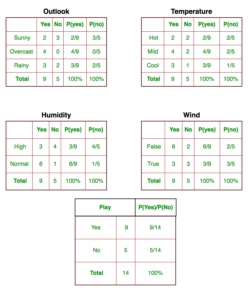
So, in the figure above, we have calculated P(x_i | y_j) for each x_i in X and y_j in y manually in the tables 1-4. For example, probability of playing golf given that the temperature is cool, i.e P(temp. = cool | play golf = Yes) = 3/9.

Also, we need to find class probabilities (P(y)) which has been calculated in the table 5. For example, P(play golf = Yes) = 9/14.

So now, we are done with our pre-computations and the classifier is ready!

Let us test it on a new set of features (let us call it today):

            today = (Sunny, Hot, Normal, False)                      

So, probability of playing golf is given by:

and probability to not play golf is given by:

Since, P(today) is common in both probabilities, we can ignore P(today) and find proportional probabilities as:

and

Now, since

These numbers can be converted into a probability by making the sum equal to 1 (normalization):

and

Since

So, prediction that golf would be played is 'Yes'.

The method that we discussed above is applicable for discrete data. In case of continuous data, we need to make some assumptions regarding the distribution of values of each feature. The different naive Bayes classifiers differ mainly by the assumptions they make regarding the distribution of P(x_i | y).

Now, we discuss one of such classifiers here.

Gaussian Naive Bayes classifier

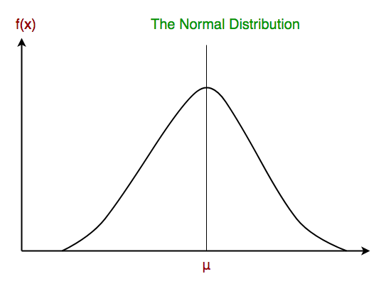
In Gaussian Naive Bayes, continuous values associated with each feature are assumed to be distributed according to a Gaussian distribution. A Gaussian distribution is also called Normal distribution. When plotted, it gives a bell shaped curve which is symmetric about the mean of the feature values as shown below:

The likelihood of the features is assumed to be Gaussian, hence, conditional probability is given by:

Now, we look at an implementation of Gaussian Naive Bayes classifier using scikit-learn.

from sklearn.datasets import load_iris

iris = load_iris()

X = iris.data

y = iris.target

from sklearn.model_selection import train_test_split

X_train, X_test, y_train, y_test = train_test_split(X, y, test_size = 0.4 , random_state = 1 )

from sklearn.naive_bayes import GaussianNB

gnb = GaussianNB()

gnb.fit(X_train, y_train)

y_pred = gnb.predict(X_test)

from sklearn import metrics

print ( "Gaussian Naive Bayes model accuracy(in %):" , metrics.accuracy_score(y_test, y_pred) * 100 )

Output:

Gaussian Naive Bayes model accuracy(in %): 95.0

Other popular Naive Bayes classifiers are:

• Multinomial Naive Bayes: Feature vectors represent the frequencies with which certain events have been generated by a multinomial distribution. This is the event model typically used for document classification.
• Bernoulli Naive Bayes: In the multivariate Bernoulli event model, features are independent booleans (binary variables) describing inputs. Like the multinomial model, this model is popular for document classification tasks, where binary term occurrence(i.e. a word occurs in a document or not) features are used rather than term frequencies(i.e. frequency of a word in the document).

As we reach to the end of this article, here are some important points to ponder upon:

• In spite of their apparently over-simplified assumptions, naive Bayes classifiers have worked quite well in many real-world situations, famously document classification and spam filtering. They require a small amount of training data to estimate the necessary parameters.
• Naive Bayes learners and classifiers can be extremely fast compared to more sophisticated methods. The decoupling of the class conditional feature distributions means that each distribution can be independently estimated as a one dimensional distribution. This in turn helps to alleviate problems stemming from the curse of dimensionality.

This blog is contributed by Nikhil Kumar. If you like GeeksforGeeks and would like to contribute, you can also write an article using write.geeksforgeeks.org or mail your article to contribute@geeksforgeeks.org. See your article appearing on the GeeksforGeeks main page and help other Geeks.

Please write comments if you find anything incorrect, or you want to share more information about the topic discussed above.

gulloarth1965.blogspot.com

Source: https://www.geeksforgeeks.org/naive-bayes-classifiers/

Share this post